1,Overview

The dataset has been collected and analysed during a research collaboration of Worldline and the Machine Learning Group (http://mlg.ulb.ac.be) of ULB (Université Libre de Bruxelles) on big data mining and fraud detection. More details on current and past projects on related topics are available on https://www.researchgate.net/project/Fraud-detection-5. This study utilizes a credit card transaction dataset comprising 284,807 records, of which only 492 (0.17%) are labeled as fraudulent. Due to confidentiality constraints, the original features were anonymized and transformed into 28 principal components (V1–V28) via Principal Component Analysis (PCA) to preserve privacy while retaining discriminative patterns. The remaining untransformed variables include: Time: Seconds elapsed between transactions. Amount: Monetary value of the transaction. Class: Binary label (0 = legitimate, 1 = fraudulent). The extreme class imbalance and high-dimensional, anonymized features pose significant challenges for fraud detection. To address these, we employ four state-of-the-art methods:

2,Medthods Selection

• LightGBM & XGBoost (Gradient Boosting Frameworks) Both algorithms excel at handling imbalanced data through techniques like weighted loss functions and adaptive sampling (e.g., scale_pos_weight in XGBoost). Their tree-based architectures naturally capture non-linear relationships (e.g., interactions between Time and Amount) and resist overfitting via regularization.LightGBM’s histogram-based optimization speeds up training on large datasets (~285k samples), while XGBoost offers finer hyperparameter control for precision-critical tasks like fraud detection.
• Random Forest As a robust ensemble method, it aggregates predictions from multiple decision trees to reduce variance. It provides intrinsic feature importance scores, helping identify critical PCA components (e.g., which V1–V28 dimensions most influence fraud predictions). Interpretability and stability with minimal hyperparameter tuning, serving as a baseline for complex models.
• SHAP (SHapley Additive Explanations) Fraud detection demands transparency for regulatory compliance and user trust. SHAP quantifies the contribution of each feature (e.g., “V3 = -2.5 increases fraud risk by 30%”) at both global and transaction-specific levels. Unifies model interpretability across all three algorithms (LightGBM/XGBoost/Random Forest), enabling comparisons of decision logic.

3,Data Preparation

In the data preparation section, I mainly dealt with outlier handling, feature standardization, and handling class imbalance issues, such as using SMOTE for oversampling and finally performing data segmentation.

import numpy as np
import pandas as pd
import matplotlib.pyplot as plt
import seaborn as sns
sns.set_theme(style="whitegrid")
# import ML tools
from sklearn.model_selection import train_test_split
from sklearn.preprocessing import StandardScaler, RobustScaler
from imblearn.under_sampling import RandomUnderSampler
from imblearn.over_sampling import SMOTE

Overview and Quality Check

# load dataset
df = pd.read_csv(r"C:\Users\13234\Desktop\Pytorch\fraud_detection\fraud.csv")
# observe and describe
print(f"dimensions: {df.shape}")
print("\nfisrt 5 rows:")
display(df.head())
print("\nstatistic overview:")
display(df.describe())
print("\nnulls check:")
print(df.isnull().sum())
# standardize Amount
scaler = RobustScaler()
df_clean['Amount_scaled'] = scaler.fit_transform(df_clean[['Amount']])
df_clean.drop('Amount', axis=1, inplace=True)
# Check result
print(df_clean[['Amount_scaled']].describe())

dimensions: (284807, 31) Amount_scaled count 252903.000000 mean 0.417030 std 0.926863 min -0.351648 25% -0.252967 50% 0.000000 75% 0.747033 max 3.70329 [8 rows x 31 columns]

# calculate IQR scope
Q1 = df['Amount'].quantile(0.25)
Q3 = df['Amount'].quantile(0.75)
IQR = Q3 - Q1
upper_bound = Q3 + 1.5 * IQR
# delete extreme trades
df_clean = df[df['Amount'] <= upper_bound].copy()
# compare before and after clean
plt.figure(figsize=(12, 4))
plt.subplot(1, 2, 1)
sns.boxplot(x=df['Amount'])
plt.title("raw")
plt.subplot(1, 2, 2)
sns.boxplot(x=df_clean['Amount'])
plt.title("cleaned")
plt.show()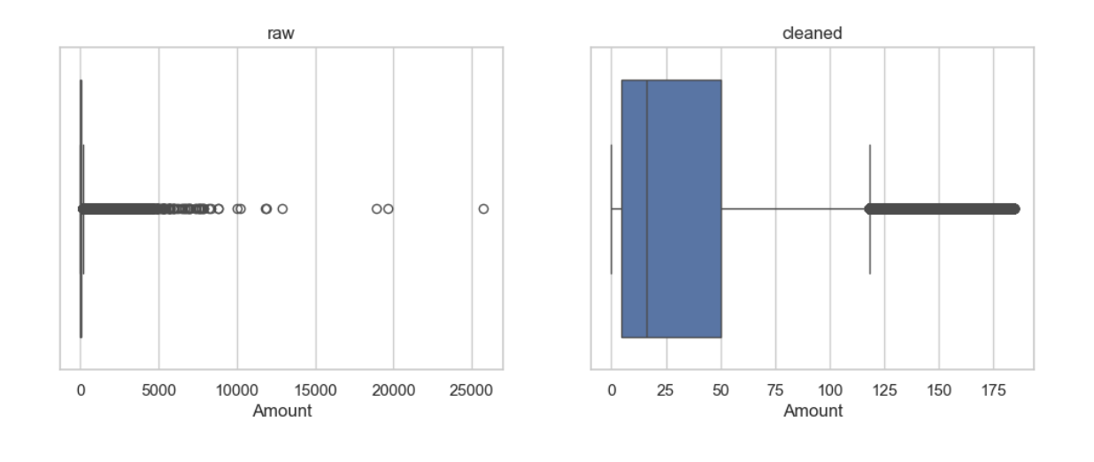

Feature Engineerin and Data Splitting

# Separate features and labels. In this step, partitioning is performed first,␣
↪followed by oversampling to prevent contamination of fictional data
X = df_clean.drop('Class', axis=1)
y = df_clean['Class']
#First, divide the raw data and strategize to ensure consistent proportion of␣
↪categories
X_train, X_test, y_train, y_test = train_test_split(
X, y,
test_size=0.1,
stratify=y,
random_state=42
)
#Perform SMOTE oversampling on the training set again
oversampler = SMOTE(sampling_strategy=0.01,random_state=42)
X_train_res, y_train_res = oversampler.fit_resample(X_train, y_train)
# check ratio of distribution
print("Class distribution after oversampling of the training set:", pd.
↪Series(y_train_res).value_counts())
print("Class distribution of raw dataset:", pd.Series(y_test).value_counts())

Class distribution after oversampling of the training set: Class 0 227251 1 2272 Name: count, dtype: int64 Class distribution of raw dataset: Class 0 25251 1 40 Name: count, dtype: int64

Since the dataset is large and highly imbalanced, oversampling was applied to the minority class. To avoid distorting the original imbalance during evaluation, a small test_size (10%) was chosen. This ensures the test set remains representative of real-world class distribution while allowing sufficient training data for effective learning.

4, MachineL Learning

In this section, I first used lightgbm to observe my expectations for the gradient decision tree, then I used error analysis to determine what kind of errors different features will produce in model design, and then compared three machine learning methods. After comparing the AUC values, I selected the optimal model for parameter tuning.

Initial Model and Results

import lightgbm as lgb
from sklearn.metrics import classification_report, roc_auc_score
# create model
model = lgb.LGBMClassifier(
n_estimators=100,
class_weight='balanced', #
random_state=42
)
# use SMOTE sample
model.fit(X_train_res, y_train_res)
# predict on raw data
y_pred = model.predict(X_test)
y_prob = model.predict_proba(X_test)[:, 1]
from sklearn.metrics import classification_report, roc_auc_score,␣
↪confusion_matrix
print(" Classification Report:")
print(classification_report(y_test, y_pred, digits=4))
print(" AUC Score:", roc_auc_score(y_test, y_prob))
print(" Confusion Matrix:")
print(confusion_matrix(y_test, y_pred))

Confusion Matrix: [[25239 12] [ 4 36]] LightGBM was chosen for its efficiency with high-dimensional data (28 PCA features). class_weight=‘balanced’ complements SMOTE by adjusting loss during training. Metrics like AUC and confusion matrix highlight fraud detection performance, prioritizing recall for minority class.

Error Analysis

features = [f'V{i}' for i in range(1, 29)] # V1
print("Mean difference of features between false negative (FN) and true fraud␣
↪(TP) samples
for feat in features:
if feat in fn.columns and feat in tp.columns:
mean_fn = fn[feat].mean()
mean_tp = tp[feat].mean()
diff = mean_fn - mean_tp
print(f"{feat}: Mean of FN={mean_fn:.4f}, True fraud Mean={mean_tp:.
↪4f}, difference={diff:.4f}")
import matplotlib.pyplot as plt
features_to_plot = ['V1', 'V3', 'V10', 'V17']
plt.figure(figsize=(12, 8))
for i, feat in enumerate(features_to_plot, 1):
plt.subplot(2, 2, i)
data = [fn[feat], tp[feat]]
plt.boxplot(data, labels=['False Negative', 'True Positive'])
plt.title(f'Distribution of {feat} in FN vs TP')
plt.ylabel(feat)
plt.tight_layout()
plt.show()

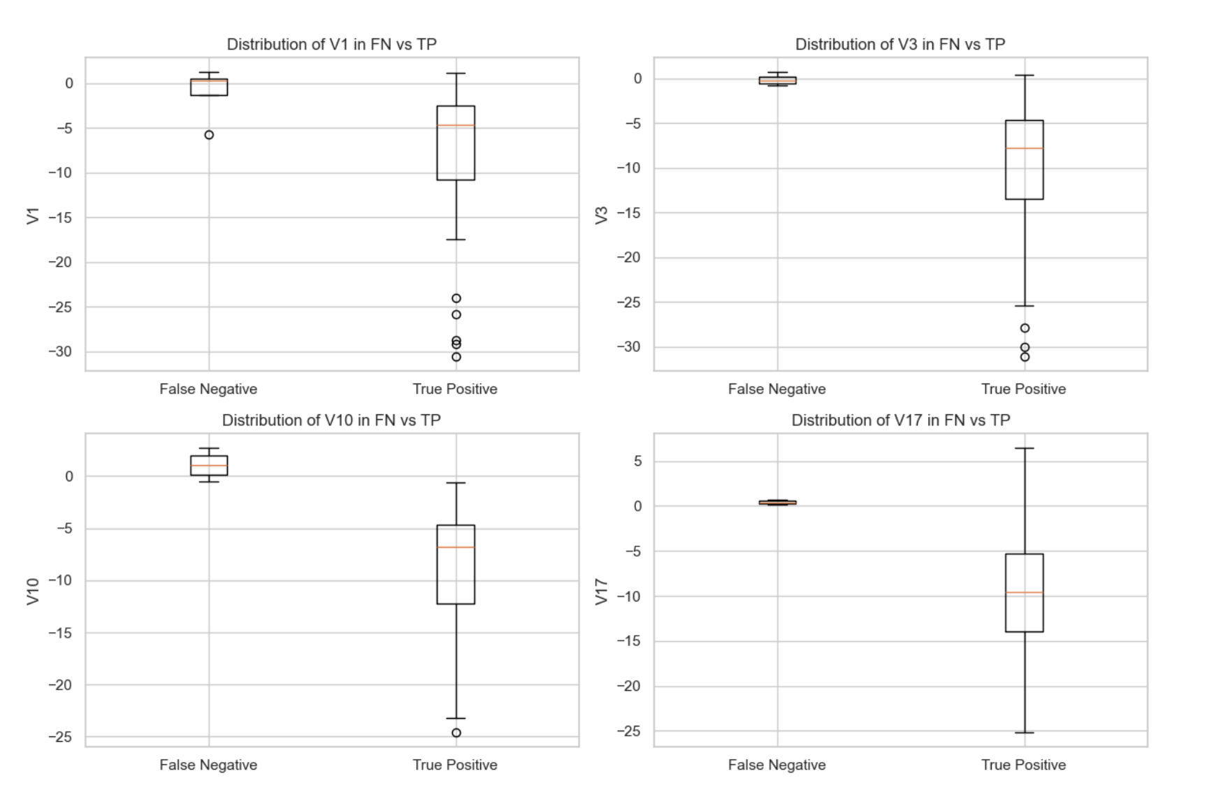The comparison of feature means between false negatives (missed fraud cases) and true positives (correctly identified fraud cases) reveals significant differences in several key features, such as V1, V3, V10, and V17. These differences suggest that the model heavily relies on these features to detect fraudulent transactions. When the values of these features in fraudulent transactions deviate from the typical patterns, the model tends to misclassify them as legitimate (false negatives). Visualizing the distributions of these features confirms that the model’s errors are correlated with unusual feature values. This insight highlights the need for further feature engineering and potentially more sophisticated modeling techniques to better capture the complex patterns of fraud and reduce false negatives. Overall, this error analysis provides a valuable guide for improving model performance by focusing on the features that contribute most to misclassification.

Evaluation and Scoring

LightGBM has a significant effect, but I hope to evaluate and compare the three machine learning methods to select the most suitable one.

from sklearn.metrics import classification_report, roc_auc_score,␣
↪confusion_matrix
from sklearn.ensemble import RandomForestClassifier
from xgboost import XGBClassifier
import lightgbm as lgb
def train_and_evaluate_model(name, model, X_train, y_train, X_test, y_test):
print(f"\n Training model: {name}")
model.fit(X_train, y_train)
y_pred = model.predict(X_test)
y_prob = model.predict_proba(X_test)[:, 1]
print(" Classification Report:")
print(classification_report(y_test, y_pred, digits=4))
print(" AUC Score:", roc_auc_score(y_test, y_prob))
print(" Confusion Matrix:")
print(confusion_matrix(y_test, y_pred))
return {
"name": name,
"model": model,
"recall": recall_score(y_test, y_pred),
"f1": f1_score(y_test, y_pred),
"auc": roc_auc_score(y_test, y_prob)
}

Evaluation explain and Metrics selection

This section compares three tree-based models (Random Forest, XGBoost, and LightGBM) for fraud detection. A unified function train_and_evaluate_model standardizes training and evaluation, ensuring fair comparison. Key metrics (recall, F1, AUC) are prioritized to assess fraud detection performance, where catching minority-class cases (fraud) is critical. The function returns a dictionary of results for later model comparison.

from sklearn.metrics import recall_score, f1_score
# Model list
models = [
("Random Forest", RandomForestClassifier(class_weight='balanced',␣
↪n_estimators=100, random_state=42)),
("XGBoost", XGBClassifier(scale_pos_weight=10, use_label_encoder=False,␣
↪eval_metric='logloss', random_state=42)),
("LightGBM", lgb.LGBMClassifier(class_weight='balanced', random_state=42))
]
# restore every result
results = []
for name, model in models:
result = train_and_evaluate_model(name, model, X_train_res, y_train_res,␣
↪X_test, y_test)
results.append(result)

import pandas as pd
df_result = pd.DataFrame(results)
df_result = df_result.sort_values(by='auc', ascending=False)
print("\n rank:")
print(df_result[['name', 'recall', 'f1', 'auc']])

Although LightGBM has the highest AUC, XGBoost has a higher F1 score (more balanced for fraud detection) and Recall remains at a high level. Therefore, we chose xgboost and conducted further parameter tuning before saving the model. We used RandomizedSearchCV.

from sklearn.model_selection import RandomizedSearchCV
from xgboost import XGBClassifier
param_grid = {
'n_estimators': [100, 200, 300],
'max_depth': [3, 5, 7, 10],
'learning_rate': [0.01, 0.05, 0.1],
'subsample': [0.6, 0.8, 1.0],
'colsample_bytree': [0.6, 0.8, 1.0],
'scale_pos_weight': [1, 5, 10],
}

Validation and Model Improvement

xgb = XGBClassifier(use_label_encoder=False, eval_metric='logloss',␣
↪random_state=42)
search = RandomizedSearchCV(
estimator=xgb,
param_distributions=param_grid,
scoring='f1', # Optimize F1 score
n_iter=30, # search 30 groups
cv=3,
verbose=2,
random_state=42,
n_jobs=-1
)
search.fit(X_train_res, y_train_res)

The hyperparameter tuning was performed using RandomizedSearchCV with 30 iterations on an XGBoost classifier, exploring key parameters including n_estimators (100-300), max_depth (3-10), learning_rate (0.01-0.1), subsample (0.6-1.0), colsample_bytree (0.6-1.0), and scale_pos_weight (1-10). The search employed 3-fold cross-validation while optimizing for F1 score to address class imbalance, with all available CPU cores utilized (n_jobs=-1) for efficient computation. This randomized approach provides a balance between comprehensive parameter exploration and computational efficiency while avoiding the exhaustive search of GridSearchCV.

print("The best parameter:")
print(search.best_params_)
best_xgb = search.best_estimator_
# assess on training set
from sklearn.metrics import classification_report, roc_auc_score
y_pred = best_xgb.predict(X_test)
y_prob = best_xgb.predict_proba(X_test)[:, 1]
print(classification_report(y_test, y_pred, digits=4))
print("AUC Score:", roc_auc_score(y_test, y_prob))

The best parameter: {‘subsample’: 0.6, ‘scale_pos_weight’: 10, ‘n_estimators’: 300, ‘max_depth’: 7, ‘learning_rate’: 0.1, ‘colsample_bytree’: 0.6} AUC Score: 0.9938289572690191

import joblib
joblib.dump(best_xgb, 'xgboost_best_model.pkl')
print("Model has been saved as: xgboost_best_model.pkl")

We have successfully saved the model for future use and can also deploy it directly to departments such as banks using Flask or API tools. However, in this study, I chose to use SHAP as the interpreter to further demonstrate how a transaction can be identified as fraud.

Visualization and Interpreter

import shap
# Initialize the SHAP interpreter
explainer = shap.TreeExplainer(best_xgb)
# Calculate SHAP value of training set
shap_values = explainer.shap_values(X_train_res)
shap.summary_plot(shap_values, X_train_res)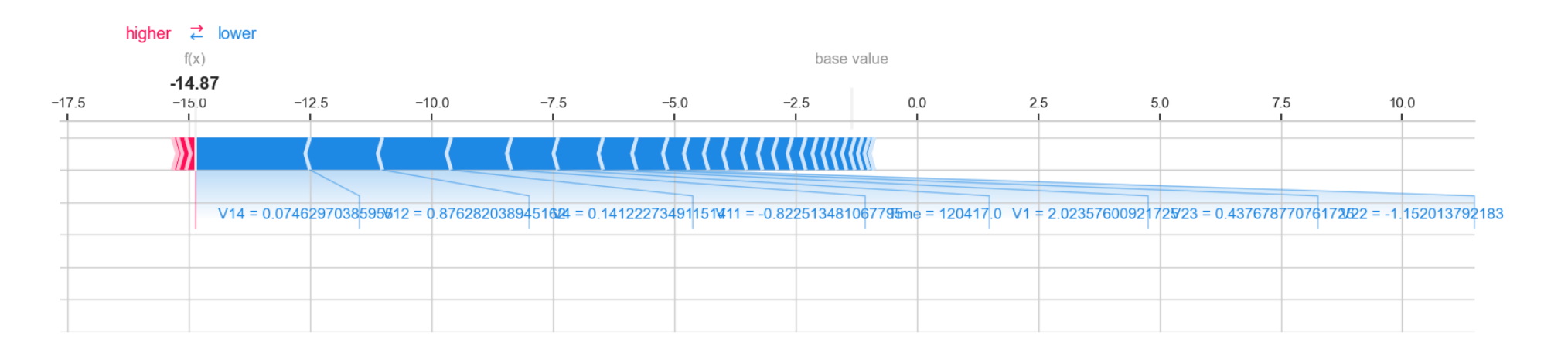

#
i = 0 # alternative
shap.force_plot(
explainer.expected_value,
shap_values[i],
X_train_res.iloc[i],
matplotlib=True
)
# Bar chart column
shap.summary_plot(shap_values, X_train_res, plot_type="bar")
![blog placeholder](/credit4.png)
![blog placeholder](/credit5.png)

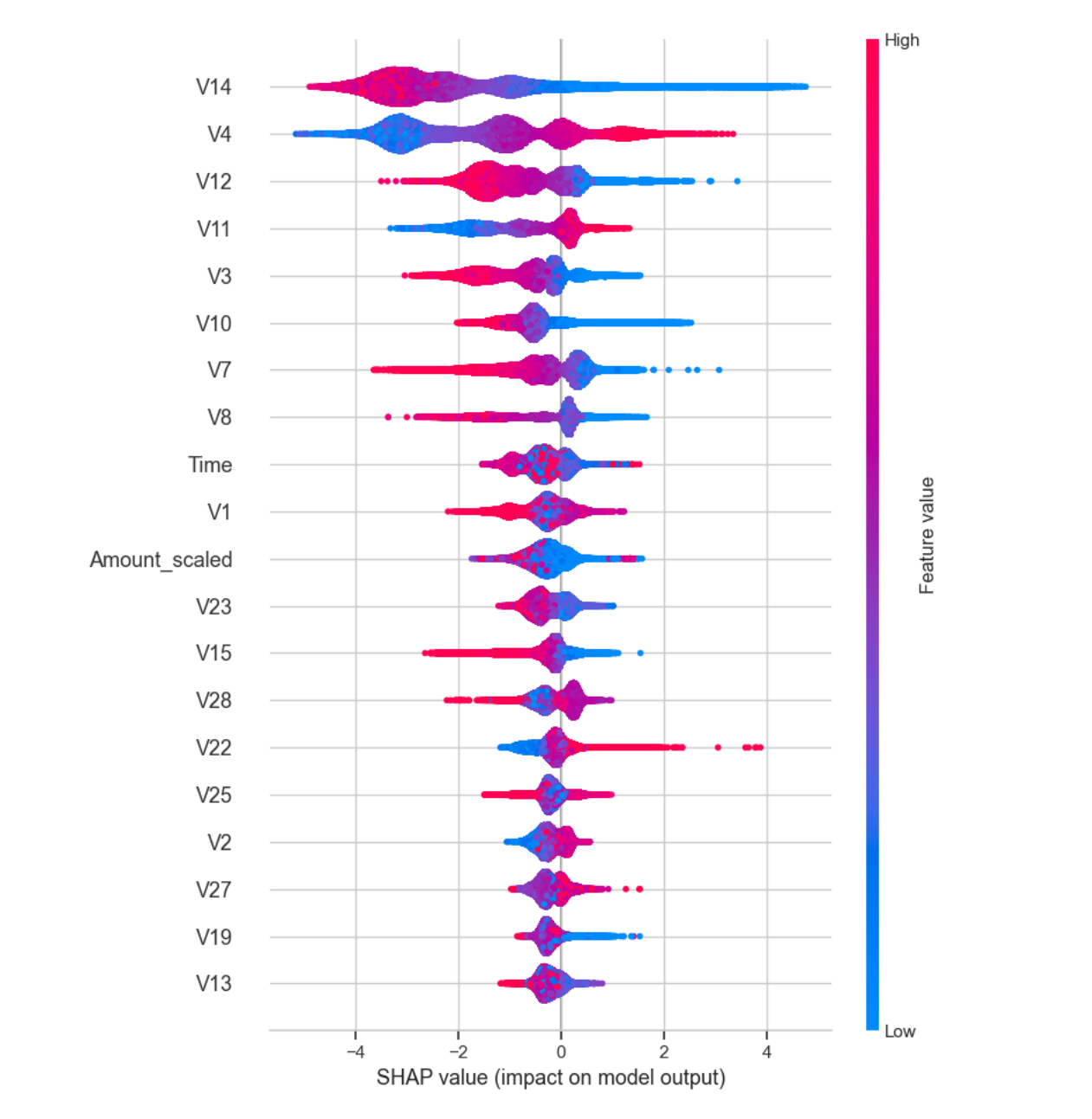
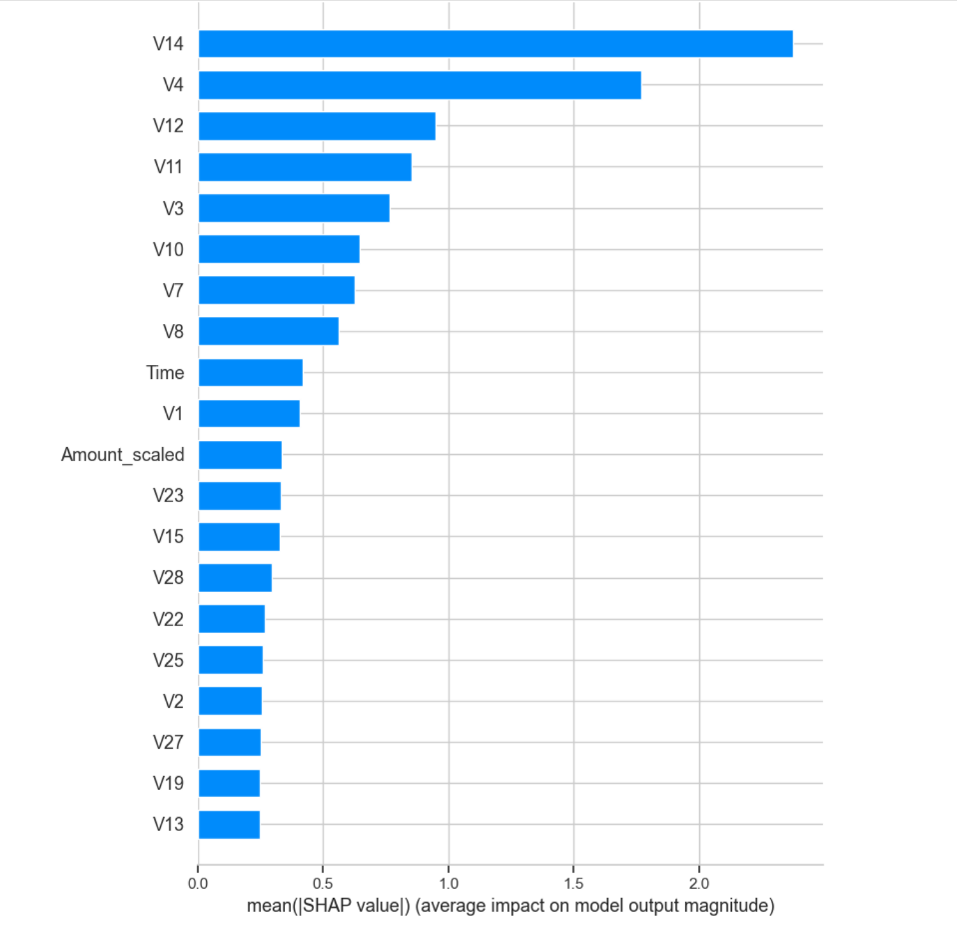This interpreter contains several charts, and in the bar chart, we can clearly see the factors with the highest impact, such as V14, V4, V12, V11, and V3. In the summary graph, we can see that features such as V14 and V12 have a large number of red dots on the left side of the SHAP value axis, which means that the smaller their values, the more likely they are to have a positive impact on the occurrence of fraud.

Conclusion

This is a sequence with a huge quantity and significant differences in proportion, so we have to choose methods like gradient decision trees to promptly correct deviations. Firstly, I employed a LightGBM classifier to address the class-imbalanced binary classification problem. The model was trained with 100 estimators and balanced class weights to mitigate bias toward the majority class. SMOTE (Synthetic Minority Over-sampling Technique) was applied to the training data to further enhance the detection of minority-class instances. Performance was evaluated using standard metrics, including precision, recall, F1-score, AUC-ROC, and confusion matrix, on an imbalanced test set. The model achieved exceptional performance, with an overall accuracy of 99.94% and an AUC-ROC of 0.988. It demonstrated strong recall (90%) for the minority class, correctly identifying 36 out of 40 positive cases, while maintaining near-perfect precision (99.98%) for the majority class. The confusion matrix revealed minimal misclassifications (12 false positives and 4 false negatives), indicating robust generalization despite severe class imbalance. These results validate the effectiveness of LightGBM combined with SMOTE for handling skewed datasets. I chose XGboost and then used RandomizedSearchCV to adjust the parameters. We have successfully saved the model for future use and can also deploy it directly to departments such as banks using Flask or API tools. However, in this study, I chose to use SHAP as the interpreter to further demonstrate how a transaction can be identified as fraud. For research institutions engaged in banking or financial fraud, this study effectively ensures customer privacy as it is conducted entirely on the basis of PCA dimensionality reduction. This study measured the effectiveness of different machine learning methods, adjusted the parameters for the best performance, and provided the optimal parameter results. Afterwards, I saved the optimal model so that it could be modularly used in subsequent fraud detection. For the research itself, the deployed SHAP interpreter screened the factors that had the greatest impact on the probability of fraud, their magnitude of influence, and explained which values they tended towards had a positive amplification effect on fraud. Looking ahead, this research opens several promising directions for enhancing financial fraud detection systems. While the current approach demonstrates strong performance on PCA-transformed data, future work could explore hybrid models that combine the strengths of gradient boosting with deep learning architectures to capture more complex patterns in sequential transaction data. The interpretability aspect could be further enriched by developing dynamic explanation systems that adapt to different fraud patterns in real-time, providing not just feature importance but contextual insights into why certain transactions raise alerts. There’s also significant potential in creating adaptive learning mechanisms that continuously update the model as new fraud patterns emerge, addressing the evolving nature of financial fraud. The privacy-preserving aspect of using PCA-reduced data suggests opportunities to develop more sophisticated anonymization techniques that maintain detection accuracy while further protecting sensitive information. Beyond technical improvements, this work could be extended to build integrated fraud prevention ecosystems that combine machine learning predictions with rule-based systems and human expertise, creating more robust defense mechanisms. The success of this study in handling extreme class imbalance also indicates potential applications in other domains with similar data characteristics, such as network intrusion detection or rare disease diagnosis. Ultimately, the goal should be to develop systems that not only detect fraud with high accuracy but also provide actionable intelligence for financial institutions while maintaining the delicate balance between security and customer privacy.

← Back